on
Free Throw Bet Analysis
This post was written jointly by Max Chiswick and Mike Thompson
Contents
- The Bet
- Assumptions and Simplifications
- Probability of making 90/100
- When to reset attempts? Method 1: Binomial
- When to reset attempts? Method 2: Reinforcement Learning
- Monte Carlo Simulations
- Markov Chain
- Practical Strategy and Conclusions
The Bet
Mike McDonald is a successful gambler/poker player who set up a bet with the following terms:
Main terms:
- I must sink 90/100 free throws on an attempt. I get unlimited attempts.
- Regulation ball, regulation hoop, lane violations not allowed
- Even money
- Bet lasts until end of 2020
Detailed additions:
- I must define when an attempt starts. I.e. if I shot 150 times and scored 90/100 between attempts 20-119 I’d need to reset counter after 19 for it to count.
- If I have no safe access to a regulation hoop I get an extension until I have had 50 hours of safe use of a regulation hoop
The short version is that Mike has to make 90/100 free throws by the end of 2020 with unlimited attempts and unlimited time per attempt, but each attempt has to be declared.
Assumptions and Simplifications
It seems that the “hot hand” theory of improving chances of making a basket on a “hot streak” is pretty unclear (Wikipedia article) and also would make the analysis much more complicated, so we assume a fixed probability of making each shot (except for one section where we look specifically at the hot hand idea).
In reality, a person does not have a fixed true shooting percentage. The probability of making a shot will vary day by day and even throughout an attempt. A more accurate model would treat true shooting percentage as a random variable rather than a fixed quantity. Since success is a tail event (in the situation where the true shooting percentage is in the high 70’s), added variance around true shooting percentage will make the probability of success more likely.
There are two main elements that go into the bet: skill level and reset strategy. The skill level is defined as the probability of making each shot. The reset strategy is when to start a fresh 100 shot attempt. We suggest that if the probability of success from any point is worse than the probability of success from the starting point, then it’s best to reset. (Although in reality, it makes sense to prefer to continue when the probability is the same or slightly worse than the starting probability since it will take more time to start over.)
Probability of making 90/100
If we assume a fixed probability of making each shot equal to \(p\), then the probability of making at least 90 out of 100 shots is a binomially distributed random variable, with probability of success equal to: \(\sum_{i=90}^{100} {100 \choose i} * p^i*q^{100-i}\); where \(q\) is the probability of a miss = \(1 - p\).
We can evaluate the probability of success by plugging in various values for true shooting percentage (\(p\) in the equation above).
The graph below demonstrates the impact that true shooting percentage has on probablity of success:
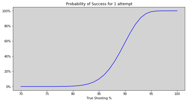
We can see that a shooter of around 70% or below is quite unlikely to ever hit 90 out of 100. Using \(p\) = 70% results in a probability of 1 in 642,853, which clearly is an unrealistic number of attempts in a one year period.
How, then, can we determine a true shooting percentage that is likely to be successful? If \(x\) equals the probability of success on one attempt (equal to the equation above), then \((1-x)\) is the probablity of failure on one attempt and \((1-x)^n\) is the probability of failure on all n attempts, then \(1-(1-x)^n\) is the probability of at least one success over \(n\) attempts.
For simplicity, let’s assume one attempt per day and again examine the probability of success for various true shooting percentages:
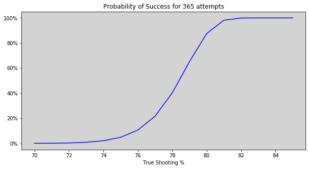 We can see that somewhere between 78% and 79% has a 50% probability of achieving success if they try 1 attempt per day. Anyone with a true shooting percentage in the low 70’s would have a marginal probability of success, and below 70% it is quite unlikely to ever make 90 out of 100 free throws. Anyone that shoots 80% or above is almost guaranteed to be successful after 365 attempts.
When to reset attempts? Method 1: Binomial
Since anyone outside of high 70’s is either almost guaranteed to fail (if below) or succeed (if above) then the question of whether he will be successful really is only interesting if his true shooting percentage falls somewhere in that range. Let’s assume a true shooting percentage of 78%, which has a 40% probability of success over 365 attempts. At what point should Mike reset his attempt back to 0 if he has missed a few shots? Obviously if he misses the first shot he should reset, and probably even if he misses the second or third shot, but what about the seventh shot? What if he is 35 of 40? One strategy is to compute the probability of success at that point in time, and reset if it is lower than his probability of success at the start of an attempt. A 78% true shooter has a 0.14% (or 1 in 709) chance of making at least 90 out of 100 free throws. If after taking \(x\) shots, he has \(y\) misses, his probability of success is: \(\sum_{i=90-x+y}^{100-x} {100-x \choose i} * 0.78^i*0.22^{100-i-x}\).
We can find the decision boundary by finding the maximum number of attempts for given number of misses \(y\) = 1 through 10 such that the probability of success is lower at that state than the probability of success at the beginning of an attempt:
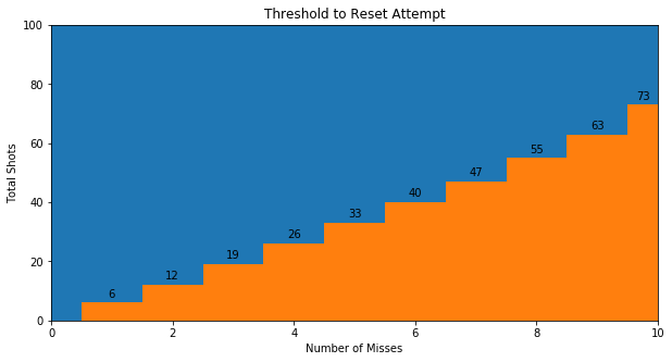
The datapoint 8 misses, 55 total attempts means that if his 8th miss was after 55 or fewer total shots, he should reset the attempt because his probability of success is lower than at the beginning of an attempt.
When to reset attempts? Method 2: Reinforcement Learning
We can analyze the reset attempt problem using reinforcement learning value iteration. Here’s how that works.
Initial definitions:
- We define a state as a pair [shots made, shots missed]
- You can think of this as a table with shots missed on the x-axis and shots made on the y-axis (see below for examples)
- Shots missed goes from 0 to 10
- Shots made goes from 0 to 90
- We define each pair to have a reward of arriving to that state of 0 except for when the bet is won, i.e. every combination where shots made = 90, so [90, 3] and [90, 5] and [90, 10], etc. all have a reward value of 100 (chosen arbitrarily to represent winning)
- We define 2 possible actions at each state: shoot or reset. These represent the actions of the player in the bet.
We want to use value iteration to find the value of every state [shots made, shots missed]. Note that the immediate reward of 100 is only given for winning the bet, so now we are defining state values that derive from that winning reward. For example, we may want to answer the question: If we are in state [85, 8] (85 shots made, 5 missed), then what is the value of being there?
Value iteration uses the Bellman equation, which is defined as \(V(s) = R(s, a) + \gamma*V(s')\), where \(V(s)\) is the value of the current state, \(R(s, a)\) is the reward of action \(a\) at state \(s\) (recall that the actions are either shoot or reset), \(\gamma\) is the discount factor, and \(V(s')\) is the value of the next state. So each state has a value for taking the “shoot” action, which is the expected value of the reward after shooting and the next state after shooting. Each state also has a value for taking the “reset” action, which is simply the value of the starting state (since there will never be a reward when resetting). The state takes the highest of the values between the two actions. In general, there is only a reward when winning the bet, so most Bellman computations have reward values of 0.
We have defined the reward for winning (i.e. 100 when shots made reaches 90) and can initially set the value of every other state at 0. Then the algorithm will learn the value of those positions. For example, if you are in the state of [89 made, 10 missed], your value is 100 if you make the next shot and you will be back to the beginning if you miss it. So we can say that the value of that state is = \(p_{make}*100 + (1-p_{make})*\text{[value of starting state]}\).
Here’s how value iteration works:
- We cycle through every combination of [shots made, shots missed] (lines 5-6)
- We set a variable \(v\) to the current value of each state (line 7)
- For each state, we evaluate the value of (1) shooting and (2) resetting (lines 9-10, calls Bellman)
- Reset is the current value of the state [0, 0]
- Shooting has a probabilistic result and we use the Bellman equation to evaluate it
- In the case of making, we have: \(make_{val} = ((p_{make})*\text{rewards[new_state_make]} + \gamma*\text{val_state[new_state_make]})\)
- In the case of missing, we have: \(miss_{val} = ((1 - p_{make})*\text{rewards[new_state_miss]} + \gamma*\text{val_state[new_state_miss]})\)
- After these calculations, we have a result for the reset action and the shoot action
- We can then set the value of the state as the result for which action gives us the greatest value (line 11)
- After each state that we check, we compare the original value of the state that we stored as \(v\) to the new value. We keep track of the largest difference as we go through each state so that at the end of the cycle, we can see what the largest difference is over all states (line 12). Once this difference converges below some \(\epsilon\) value that we define, then we consider the state values to be stable (line 14).
- Now we have values for each state, but we haven’t made a strategy (aka policy) for what to do at each state. We can iterate through every state pair one final time and check the value of each action at each state and now that these values are fixed, we can set the strategy for the state to be the action that gives the highest value. This is called policy iteration.
For the full code, see: freethrows.py
State values
Here are various figures for state values for different levels of \(p_{make}\) and \(\gamma\). The yellow areas indicate optimally continuing to shoot and the purple areas indicate optimally resetting. We also show the reset values specifically for \(p_{make}\) = 0.78 and \(\gamma\) = 0.99. The figures are clickable to see them in larger size.
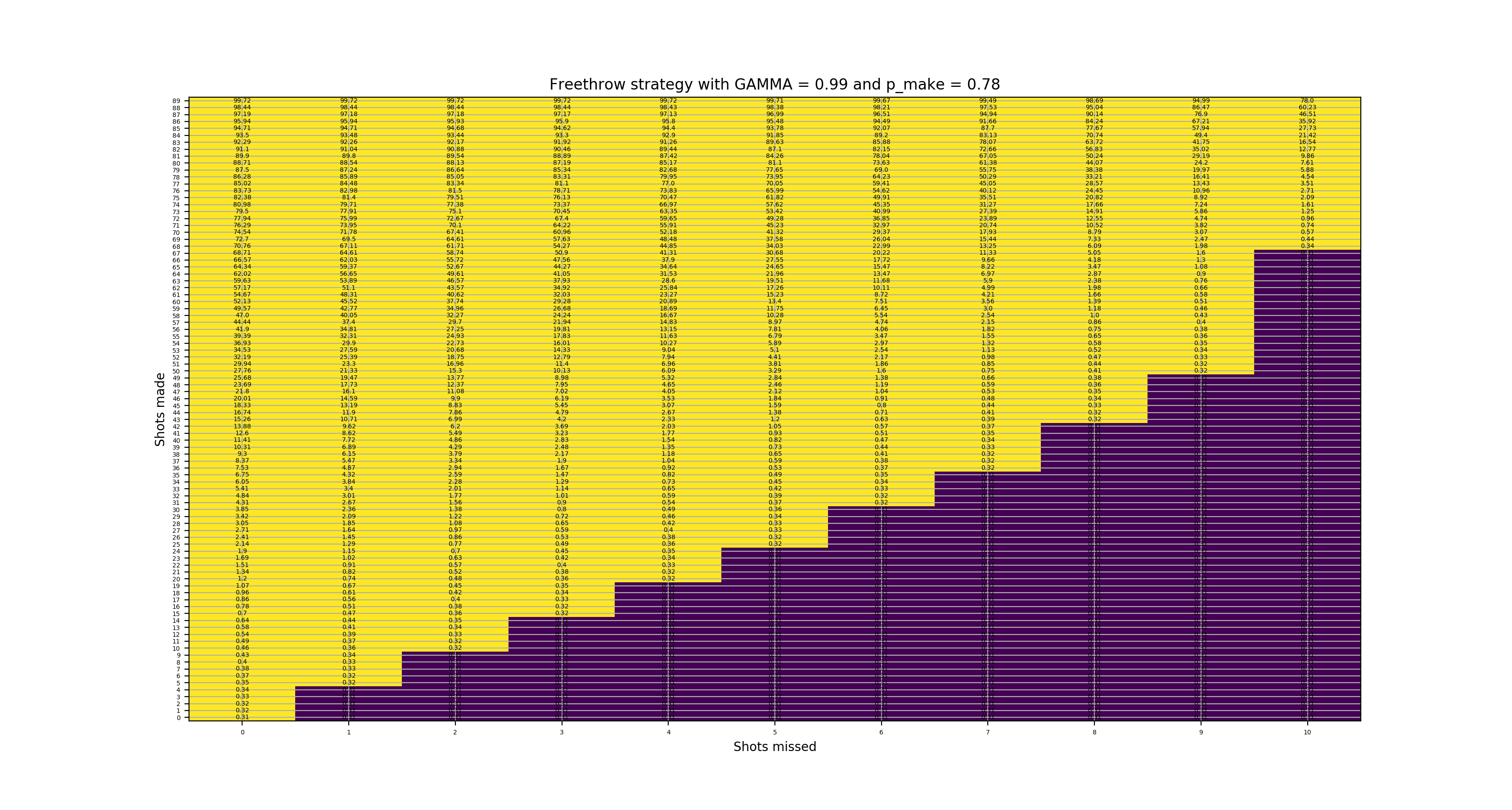
State values with 78% make
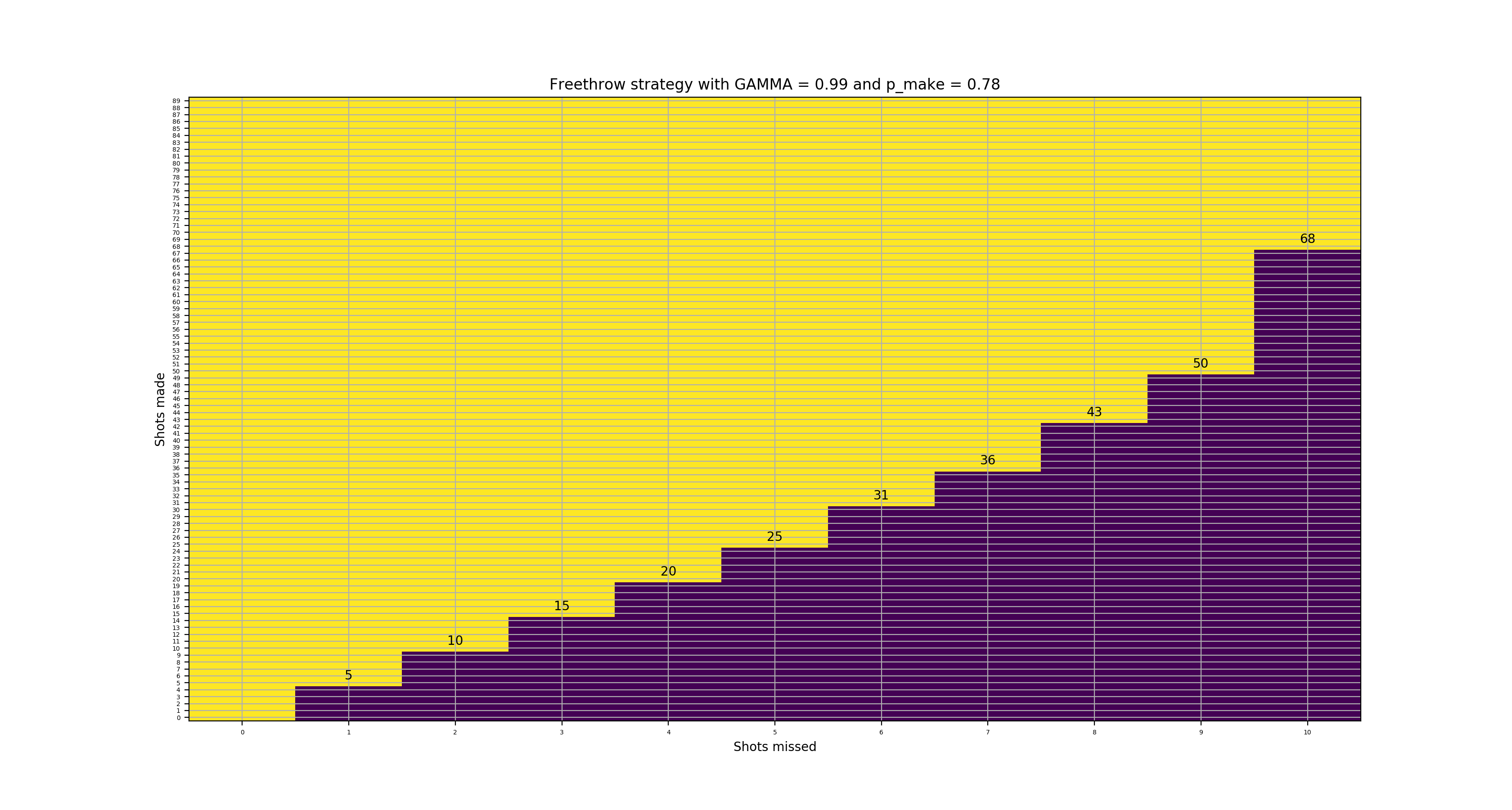
Reset values with 78% make
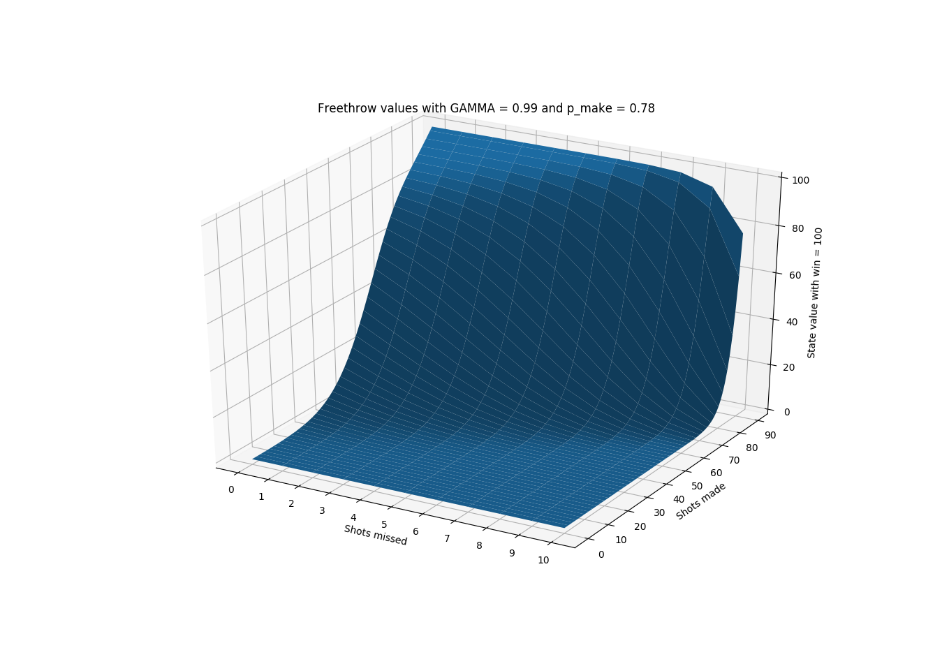
3D state values with 78% make
)
State values with 74% make
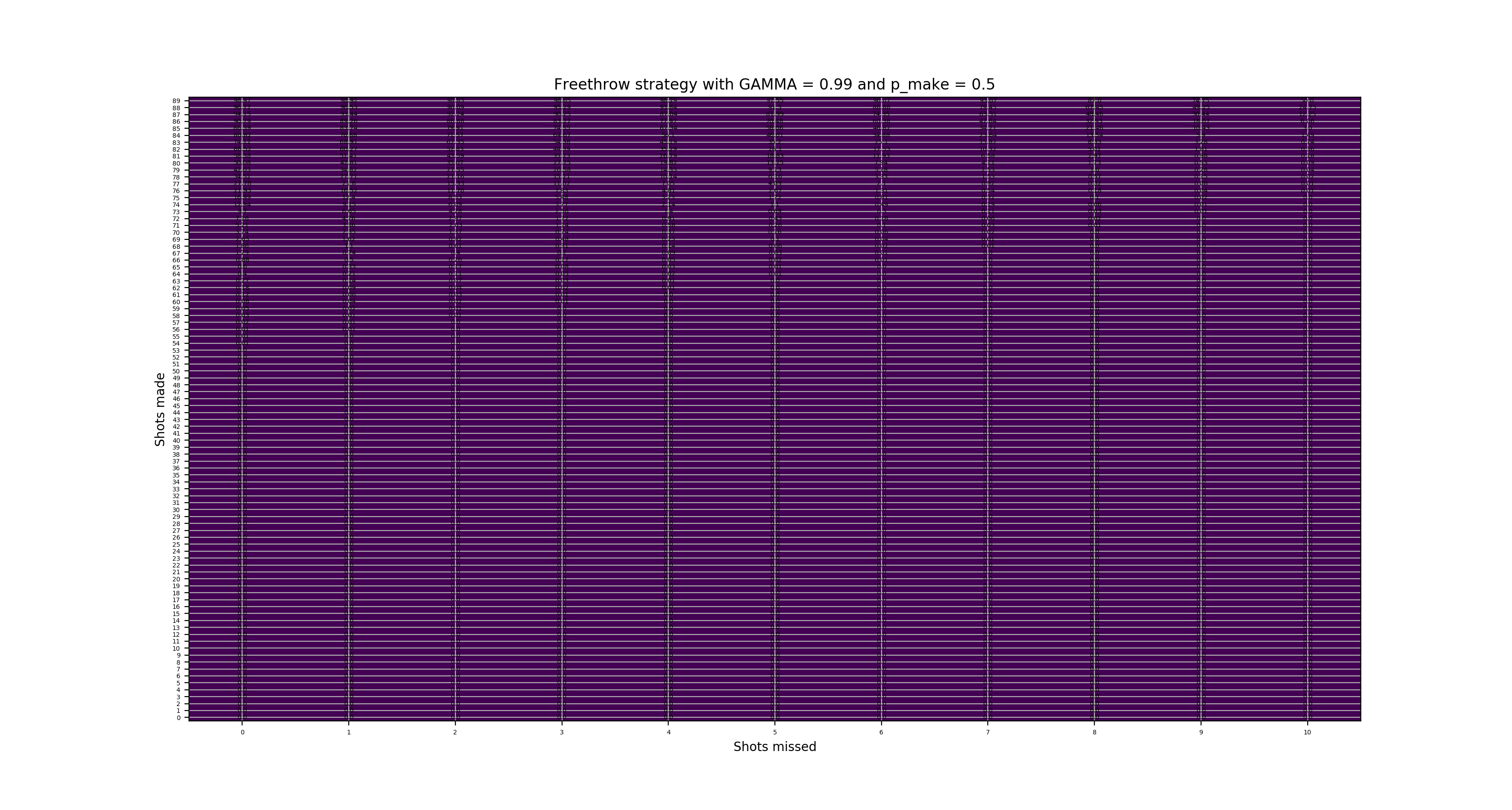
State values with 50% make
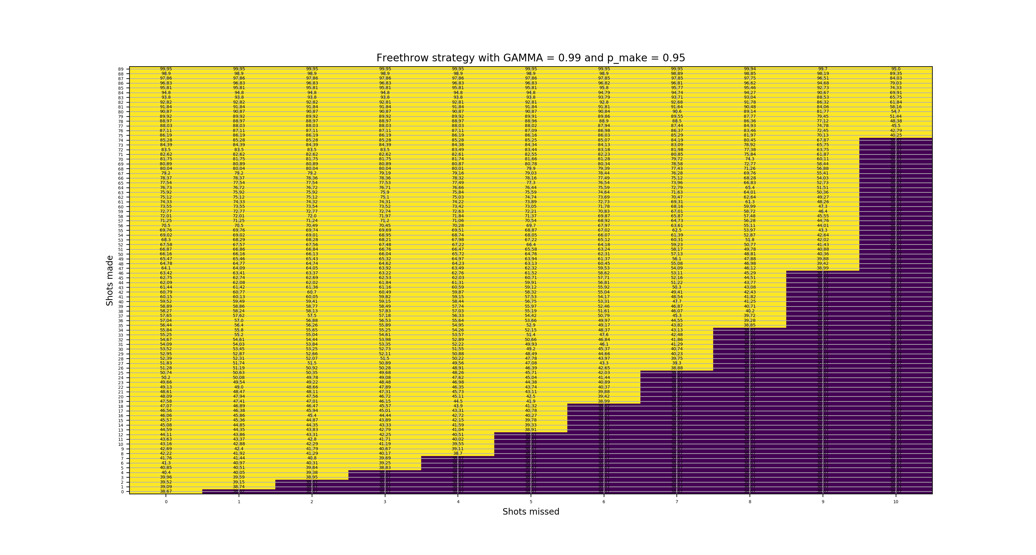
State values with 95% make
The discount rate
We use the parameter \(\gamma\) in the Bellman equation. This acts as a discount rate, which means that farther away states get discounted more compared to states nearby. We think this makes sense in the context of the free throw bet because of the time and energy required to complete attempts. For example, if we had a perfect player who could make every shot 100% of the time, if he had 1 shot left, the value of the state would be \(100 * 0.99 = 99\) and with 5 shots left would be \(100 * 0.99^5 = 95.099\) and then at the beginning with 90 shots left would be \(100 * 0.99^90 = 40.473\). So while this player’s true value is always 100, the state values include discounting to account for the time.
Going back to \(p_{make}\) = 0.78, we will show plots with \(\gamma\) = 0.999 and \(\gamma\) = 0.9, small but significant differences from the \(\gamma\) = 0.99 plot above. The \(\gamma\) = 0.9 plot “breaks” because \(0.9^{90}\) is so small that it is essentially 0 by the time the reward of winning is iterated down to the starting state.
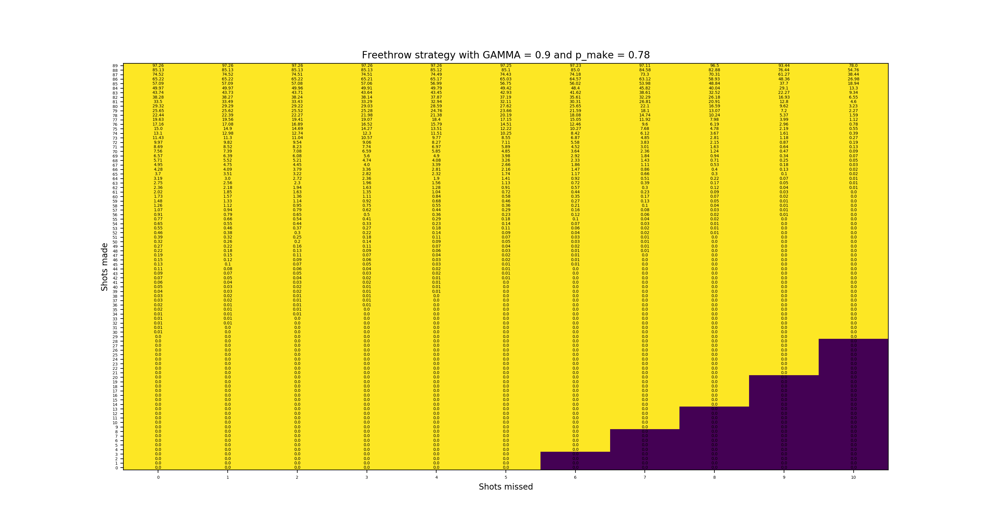
State values with 78% make and low discount factor
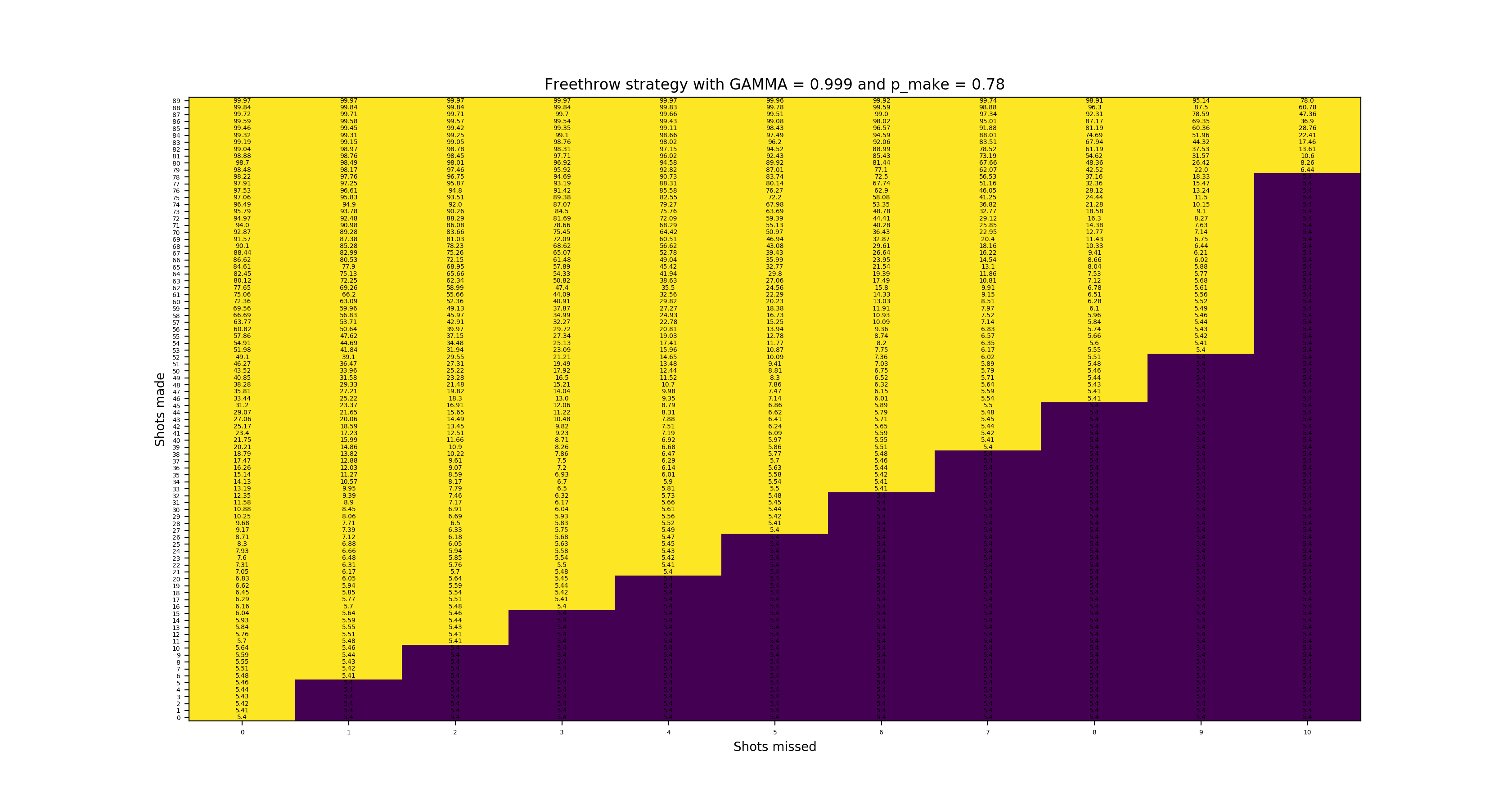
State values with 78% make and high discount factor
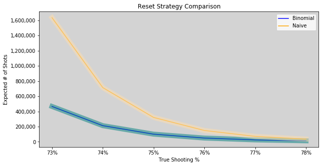
Monte Carlo Simulations
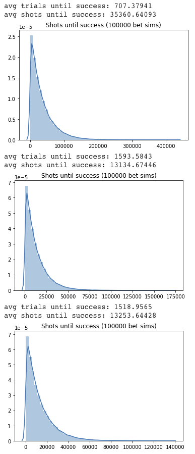
We’ve now shown a possible reset strategy that used the binomial model and a similar, but slightly different strategy that used reinforcement learning. There is also the naive strategy of just shooting until winning (making 90) or losing (missing 11). We ran Monte Carlo simulations for each of these 3 methods for 100,000 trials (where a trial is run until winning the bet). The most valuable statistic is the average number of shots until winning, which we plotted for each strategy. On top we have the naive strategy that not surprisingly has the most shots until success and in the middle is the binomial model and on the bottom is the RL model. Those are within about 1% of each other, which suggests that using a reasonable reset strategy is most important.
We did an additional Monte Carlo simulation using the binomial model 78% fixed rate reset strategy. This time we modified the shooting probabilities to a model that Mike suggested. He suggests that we model having a base free throw rate of 75%, with a floor of 65% and a ceiling of 85%. Each make elevates the current \(p_{make}\) by \(\frac{1}{4}\) towards the ceiling and each miss decreases the current \(p_{make}\) by \(\frac{1}{3}\) towards the floor.
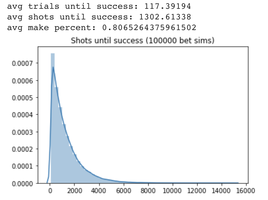
We see that \(p_{make}\) is about 80.7% on average, substantially higher than the above 78% simulations. We also see that the streakiness potential built into the shooting model allows for some very strong runs, and therefore the average shots until success goes down drastically to only 1302.6, which is about \(\frac{1}{10}\) the amount of shots under the 78% shooting with reset models and about half of the shots if we had a fixed 80.6% \(p_{make}\) (plot not shown).
Markov Chain
The free throw bet can be modeled as a Markov chain, which per Wikipedia, is: “a stochastic model describing a sequence of possible events in which the probability of each event depends only on the state attained in the previous event.”
This provides a quick way to directly calculate the average shots until success rather than doing simulations.
There are \(1001\) different possible states (\(0\) to \(10\) misses, \(0\) to \(90\) makes) \(\implies\) \(11\) * \(91\) \(=\) \(1001\). Therefore, The bet can be represented by a \(1001\) x \(1001\) matrix, where rows represent the current state, columns represent the future state, and elements \(X_{ij}\) {\(\forall\) \(_i, _j \in [0, 1000]\)} represent the probability of transitioning from state \(i\) to state \(j\).
Naive Model
Let’s assume Mike continues an attempt until either 90 makes or 11 misses, and define the states as:
\(0\), \(1\), \(\dots\), \(89\) \(=\) (\(0\) misses, \(0\) makes), (\(0\) misses, \(1\) make), \(\dots\), (\(0\) misses, \(89\) makes);
\(90\), \(91\), \(\dots\), \(179\) \(=\) (\(1\) miss, \(0\) makes), (\(1\) miss, \(1\) make), \(\dots\), (\(1\) miss, \(89\) makes);
\(\vdots\)
\(900\), \(901\), \(\dots\), \(989\) \(=\) (\(10\) misses, \(0\) makes), (\(10\) misses, \(1\) make), \(\dots\), (\(10\) misses, \(89\) makes).
\(990\), \(991\), \(\dots\), \({1,000}\) \(=\) (\(0\) misses, \(90\) makes), (\(1\) miss, \(90\) makes),\(\dots\), (\(10\) misses, \(90\) makes).
Note it will make sense later why the successful scenarios are at that end, rather than in sequential order.
Then, the probability matrix \(P\) can be fully described by:
\(X_{i,i+1}\) \(=\) \(0.78\) for {\(i\): \(i\) \(\in\) [0, 989] | (\(i\)+1)%90!=0}; (since 90 made shots are at the end rather than after 89 makes)
\(X_{89+90*i,990+i}\) \(=\) \(0.78\) for \(i\) \(\in\) [0, 10];
\(X_{i,90+i}\) \(=\) \(0.22\) for \(i\) \(\in\) [0, 899];
\(X_{900+i,0}\) \(=\) \(0.22\) for \(i\) \(\in\) [0, 89]; (reset to beginning on 11th miss)
\(X_{i,i}\) \(=\) \(1\) for \(i\) \(\in\) [990, 1,000];
\(X_{i,j}\) \(=\) \(0\) everywhere else.
\(P\) = \(\begin{array}{matrix_1} & [c_{0}] & [c_{1}] & [c_{2}] & [c_{3}] & \dots & [c_{90}] & [c_{91}] & [c_{92}] & \dots & [c_{901}] & \dots & [c_{999}] & [c_{1000}]\\ [r_{0}] & 0 & 0.78 & 0 & 0 & & 0.22 & 0 & 0 & & 0 & & 0 & 0\\ [r_{1}] & 0 & 0 & 0.78 & 0 & & 0 & 0.22 & 0 & & 0 & & 0 & 0\\ [r_{2}] & 0 & 0 & 0 & 0.78 & & 0 & 0 & 0.22 & & 0 & & 0 & 0\\ \vdots & & & & & \ddots & & & & & & \ddots & \vdots & \vdots\\ [r_{900}] & 0.22 & 0 & 0 & 0 & \dots & 0 & 0 & 0 & & 0.78 & & 0 & 0\\ \vdots & & & & & \ddots & & & & & & \ddots & \vdots & \vdots\\ [r_{999}] & 0 & 0 & 0 & 0 & \dots & 0 & 0 & 0 & & 0 & \dots & 1 & 0\\ [r_{1000}] & 0 & 0 & 0 & 0 & \dots & 0 & 0 & 0 & & 0 & \dots & 0 & 1\\ \end{array}\)
Absorbing states are states that cannot be left once entered. Then let matrix \(T\) be a subset of matrix \(P\) that only includes transition (non-absorbing) states: \(T\) = \(P_{[0:989,0:989]}\), since the final ten states represent success, completing the bet (this is the reason we set the final ten states as the success states, so they can be removed easily).
Define matrix \(C\) such that every element \(X_{ij}\) is the number of expected transitions from state \(i\) to state \(j\) at any point in time (even if other states are entered inbetween) before entering into one of the absorbing states. Matrix \(C\) is calculated as: \(C\) = (\(I_{990}\) \(-\) \(T\))\(^{-1}\). Then the sum of \(row_0\) is the expected total number of shots required for success. We calculate that under the naive assumption, where Mike shoots until the earlier of 90 makes or 11 misses, that the expected number of shots is 35,418.
Strategies from Binomial and Reinforcement Learning Models
We can modify the matrix \(P\) above to calculate the expected number of shots when Mike resets based on strategies from the binomial and reinforcement learning models. To accomplish this, we simply move the 0.22 to column 0 if the miss occurs on or before the threshold (e.g. the binomial model recommends resetting if first miss occurs within the first 6 shots, so states \(0\) through \(5\) move the probability of a miss to the first column to indicate restarting the bet).
We see that the binomial models cuts the expected number of shots down to 13,262, and the reinforcement learning model with gamma of 0.99 is a slight improvement at 13,236.
Strategy from Inspection
Since the Markov chain is fast to calculate, we can use inspection to find an even better strategy. We start by only resetting on the 10th miss. We find the value \(n_{10}\) \(\in\) (0,100) with the minimum number of expected shots. We continue to use the value found for \(n_{10}\) as the threshold for resetting on the 10th miss, and search for the threshold for resetting on the 9th miss, \(n_9 \in (0, n_{10})\) that results in the minimum expected number of shots. We continue in this manner until we have found all values \(n_ {10}, n_9, \dots, n_1\). The inspection model results in another slight improvement, with expected shots of 13,209. The thresholds to reset are if misses 1 through 10 occur on or before total number of shots: \(\)\begin{array}{inspection} 5, & 11, & 16, & 22, & 27, & 34, & 40, & 47, & 55, & 64 \end{array}\(\).
Practical Strategy and Conclusions
Mike’s shooting ability is the most important factor in whether he will be successful, with reset strategy only mattering for a rather narrow range of true shooting percentages:
To have a realistic probability of success, Mike needs to have a shooting percentage in the high 70’s or better. We think it makes sense to keep a trailing average of approximately the last 1,000 free throws as an estimate for true shooting percentage. If making less than ~75% of shots, it’s probably better to focus on improving rather than attempting the bet since more focused training would probably result in faster improvement and the chance of success is pretty low under 75%. Things like working on form (Mike already has a professional shooting coach and many at-home Twitch coaches) and conditioning and mental state all seem valuable.
As for resetting, we have shown a fairly narrow range of different reset strategies, depending on the method used to compute. It probably makes sense to have an idea of an upper/lower bound on the reset strategy and then within that range to play based on feel!